I’ve been working with research for some time now but have always found it hard to fully understand p-values, confidence intervals and statistical significance. I think this is true of many (most?) people working in social science. I thought that writing a clear explanation in my own words could help. I’m posting my attempt here for my own benefit – hopefully it leads to useful comments that improve my understanding. I’ll focus on understanding this in the context of a randomised control trial, as this is where I encounter it most often. 

I’ll try to start from first principles where I can. This means starting with the fundamental problem that p-values are designed to address: uncertainty.

Understanding uncertainty

To understand p-values and the like, we need to first adopt a particular way of thinking about RCTs. According to this way of thinking, we do RCTs because we want to know the impact of an intervention on an outcome for a population. For example, this could be the impact of a reading programme on the reading ability of all children in primary schools. But to estimate the impact on our population we need to do several things which introduce uncertainty and make it impossible to get a perfect estimate.

Usually, it’s not practically possible to do research on a whole population. We can’t do an RCT on all children in all primary schools so we need to select a smaller number of children to work with. This smaller number of children is called a sample. There is always going to be a possibility that the sample we take is different in some important way to our population. Perhaps the children in the sample respond unusually well to the intervention compared to the population as a whole. This introduces uncertainty about whether our RCT provides a good estimate of the effect of the intervention for our population. This type of uncertainty is called sampling uncertainty.

Running an RCT requires you to randomly assign some participants to an intervention group and others to a control group. We use random assignment to try to ensure that the only difference between the control and intervention groups is whether or not they receive the intervention. However, we can’t guarantee that this has been successful. There is still the risk that intervention and control groups are different in an important way. Perhaps the control group is full of participants who, for some reason unrelated to the intervention, will make smaller gains in the outcome. For example, perhaps the control group in our example RCT includes a greater number of children who have reading difficulties. This introduces the chance that any effect in the RCT is not caused by the intervention but is instead related to other differences between the two groups. This type of uncertainty is called allocation uncertainty.

A final type of uncertainty is introduced because, to make a comparison between the intervention and control groups, we need to measure outcomes for both groups. In our example RCT we’ll use a reading test to try to understand children’s reading ability. This reading test can’t give us a perfect picture of a child’s reading ability as reading ability is just too complex a concept to capture perfectly in a one-hour reading test. Every measurement we take is going to differ in some way from the ‘true’ picture of the child’s reading ability. This type of uncertainty is called measurement uncertainty.

So this is the problem that p-values and associated statistics are trying to solve. Every time we estimate the effect of an intervention in an RCT, we will face uncertainty about the effect. These statistics aim to help us think through the uncertainty around that estimate of effect. 

Sampling distribution

Before we get to p-values and confidence intervals, we’re going to have to understand some key concepts.

In part one we talked about how uncertainty is introduced when we take samples from our population. Imagine if we took lots of samples from our population. And we conducted an RCT with each sample. We could calculate an effect size for each sample. Thanks to the sources of uncertainty we discuss earlier, the effect sizes wouldn’t all be the same, they would vary.

We could plot the distribution of effect sizes on a graph and it will look something like this.

This distribution is called the sampling distribution. The graph has a bell shape – the distribution of effect sizes follows a particular type of distribution called a normal distribution. We can calculate the mean of this distribution as well as its standard deviation.

In the real world, this isn’t something we tend to be able to plot. We don’t repeat the experiment many times, with different samples. Rather we tend to take one sample and one sample only. So if we want to know the standard deviation of the sampling distribution of the effect size we have to estimate it. This estimate of the standard deviation of the sampling distribution is called the standard error. The only information we have available to calculate the standard error is from our one sample. We haven’t taken lots of samples to run lots of experiments so we must calculate the standard error from our one sample. Here’s the formula: 

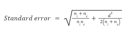
I found it useful to see this formula as it helped me realise there’s nothing especially magical or complicated about the standard error. It uses three pieces of information about the experiment sample: the effect size (d), the sample size of the intervention group (n_i) and the sample size of the control group (n_c). Larger sample sizes and effect sizes will result in a smaller standard error. 

I think it’s important to leave this section with these two key points in mind: 

• The sampling distribution is the distribution of effect sizes from multiple repeated experiments using samples drawn from the same population
• The standard error is an estimate of the standard deviation of the sampling distribution. 

Testing hypotheses

When we are working with p-values etc we are trying to test a hypothesis that the ‘true’ effect in the population is a certain size. We test this hypothesis using the sample data we collected. This hypothesis is often called the study hypothesis or the test hypothesis. Usually, the test hypothesis is that the effect size is zero – the intervention did not have an impact on our outcome of interest. In this case the test hypothesis is often called the ‘null hypothesis’.

However, the null hypothesis is not the only hypothesis we can test. We might also test the hypothesis that the effect size is 0.1 or 0.2 or any other size we can imagine. We might also test the hypothesis that it’s greater or less than a certain number, or within a certain range.

P-values

Now we can try to understand p-values. 

We have run our experiment on the reading intervention and calculated an effect size of 0.2 using our data. We now want to test a hypothesis against this data. When calculating a p-value we are usually testing the null hypothesis (i.e. that there was no effect). 

Let’s imagine that the null hypothesis is the true effect in the population – our intervention is ineffective. If we run our experiment lots of times, then the most common result in experiments will be to find no effect. I.e. the mean of the sampling distribution will be zero. But due to the sources of uncertainty mentioned above we’ll often find in individual samples that experiments produce effect sizes different to zero. If you look at the graph of the sampling distribution above there are many samples that produced quite large effects even though the true population effect is zero. 

When we calculate a p-value we start by imagining this imaginary situation where the null hypothesis is the true effect. We then ask, given that the null is true, how likely is an effect equal to or larger than the one we saw in our real experiment? This is what the p-value is: the probability that, given that the null is the true effect, we would see an effect as extreme as the one we actually saw in our data. 

So, p = 0.01 means that an effect as large as the one we observed would be unlikely to occur if the null hypothesis is true. P = 0.9 means that an effect as large as the one we observed would be likely to occur if the null hypothesis is true. 

This means that most of the common conceptions of what a p-value is are wrong. The p-value is not: 

• The probability that the effect size is the result of random chance. This can’t be true. The p-value is calculated using the assumption that the observed effect size is indeed the result of random chance (i.e. the null hypothesis is true and there is no effect). 
• The probability the intervention had an effect. Instead, the p-value is based on the assumption that the intervention did not have an effect and is the probability that you’d see results as extreme as the results you saw. 
• The probability that the observed effect size is true or false. The p-value only gives you an indication of how likely results as extreme as your observed effect are if the null hypothesis is true. You need to think about a lot more to make a strong claim about the truth of an effect. Was the study well-designed and implemented? How do your results compare to the existing evidence?  

These are all things we would love to know, but unfortunately are not easy to find out!

Here’s a final attempt at the plainest explanation of what a p-value tells us. P-values answer the question: ‘How rare would results as extreme as these be in a world where the intervention had no effect?’

Statistical significance

P-values can take any value between 0 and 1. However, researchers do not typically focus on their absolute value. They tend to focus on whether they are smaller or large than a threshold of 0.05. If the p-value is equal to or less than 0.05 then the effect is declared to be ‘statistically significant’. If the p-value is greater than 0.05 then the effect is declared to be ‘not statistically significant’. 

Too often if a result is statistically significant this is understood to mean that the effect was ‘true’. But this isn’t what it means. A small p-value means that the data is unusual if the null hypothesis and other assumptions used to calculate the p-value are correct. The p-value could be small due to large random error or problems with some of the assumptions used to calculate it. 

Aside from the misconceptions about what it  means there are some more fundamental problems with the convention of comparing p-values to a threshold for statistical significance. The choice of 0.05 as the threshold for statistically significance is arbitrary and recently statisticians have argued for it to be discontinued. Instead, if we use p-values, we should interpret them on a continuum. There’s basically no difference between p=0.04 and p=0.06 but there’s an important difference between p=0.04 and p=0.40. Most importantly, p-values should be interpreted as one of several sources of information about the study. Too often, it’s the only statistic that seems to determine our interpretation of the results. Too many studies seem to claim that a statistically significant result is true, regardless of other important aspects of the study such as its design and implementation.